Factorized Diffusion: Perceptual
Illusions by Noise Decomposition

University of Michigan
Correspondence to: ude.hcimu@gnegd

tl;dr: We can control components of generated
images with a pretrained diffusion model. We
use this to generate various perceptual illusions.

Hybrid Images

Our method can produce hybrid images, which change appearance depending on the distance (or size) at which they are viewed. These images were first proposed by Oliva et al. [1]. We do this by conditioning low and high frequency components with different text prompts. For more examples, please see our hybrid images gallery.

* Note, we aren't playing any tricks here. The only thing we're doing is changing the size of the images. You can get the same effect by standing really really far from your screen or just squinting your eyes.

* Also note, we've thrown a few "inverse hybrids" in the above video.

Color Hybrids

Our method can also make what we call color hybrids: images that change appearance when color is added or subtracted. Interestingly, because the human eye cannot see color under dim lighting, there is a physical mechanism for this illusion—these images change appearance when taken from a brightly lit environment to a dimly lit one. These images are generated by conditioning grayscale and color components on differnt prompts. For more examples, please see our color hybrids gallery.

Motion Hybrids

We can also make images that change appearance when motion blurred, which we call motion hybrids. To make these, we condition a motion blurred component on one prompt, and the residual component on another. Note in the below visualizations we synthetically add motion blur. For more examples, please see our motion hybrids gallery.

Hybrids from Real Images

In addition, we can make hybrid images from real images. We do this by taking high or low pass components from a real image, and generating the missing component. Effectively, this is a method to solve inverse problems, which we discuss in more detail below. For more examples, please see our inverse hybrids gallery.

Triple Hybrids

Finally, we can make hybrid images with three different interpretations by conditioning three different levels of a Laplacian pyramid on different prompts. We found that this was fairly difficult to do, and required manually hand tuning the Laplacian pyramid parameters. If you have difficulty seeing the prompts please try zooming in and out, or stepping a couple meters away from the screen. For more examples, please see our triple hybrids gallery.

Overview

Given a factorization of an image into a sum of components, we present a zero-shot method to independently control these components through diffusion model sampling. For example, decomposing an image into low and high spatial frequencies, and then prompting these components on different text prompts allows us to produce hybrid images. A decomposition into grayscale and color components results in images that change appearance when colored is added or subtracted. We also show how to make perceptual illusions involving motion blur and hybrid images with three prompts. Finally, by holding one component constant while generating the other components we can create hybrid images from real images.

Method

Given an image decomposition, we control components of the decomposition through text conditioning during image generation. To do this, we modify the sampling procedure of a pretrained diffusion model. Specifically, at each denoising step, \( t \), we construct a new noise estimate, \(\tilde\epsilon\), to use for denoising, whose components come from components of \(\epsilon_i\), which are noise estimates conditioned on different prompts. Here, we show a decomposition into three frequency subbands, used for creating triple hybrid images, but we consider a number of other decompositions, which we explain below.

Decompositions

In order to use our method we need to find image decompositions of the form \( \mathbf{x} = \sum f_i(\mathbf{x}) \). Below, we briefly describe the decompositions that we consider, and what kinds of images they produce.

Hybrid Decomposition

To make hybrid images, we can decompose an image into high and low frequency components. We use a low pass filter, implemented as a Gaussian blur, \( G_\sigma \), with standard deviation \( \sigma \) as one component, and we take the residual high pass as the other component. \[ \begin{aligned} \mathbf{x} = \underbrace{\mathbf{x} - G_\sigma(\mathbf{x})}_{f_\text{high}(\mathbf{x})} + \underbrace{G_\sigma(\mathbf{x})}_{f_\text{low}(\mathbf{x})} \end{aligned} \]

Triple Hybrid Decomposition

To make triple hybrid images we decompose an image as a three layer Laplacian pyramid where we use two Gaussian blurs of standard deviation \(\sigma_1\) and \(\sigma_2\). \[ \begin{aligned} \mathbf{x} &= \underbrace{G_{\sigma_1}(\mathbf{x}) - G_{\sigma_2}(G_{\sigma_1}(\mathbf{x}))}_{f_\text{med}(\mathbf{x})} \;+ \\ &\underbrace{\mathbf{x} - G_{\sigma_1}(\mathbf{x})}_{f_\text{high}(\mathbf{x})} + \underbrace{G_{\sigma_2}(G_{\sigma_1}(\mathbf{x}))}_{f_\text{low}(\mathbf{x})} \end{aligned} \]

Color Space Decomposition

To make color hybrids, we take the grayscale image as one component, and the residual as the color component. \[ \begin{aligned} f_\text{gray}(\mathbf{x}) &= \frac{1}{3} \sum_c \mathbf{x}_c \\ f_\text{color}(\mathbf{x}) &= \mathbf{x} - f_\text{gray}(\mathbf{x}) \end{aligned} \]

Motion Blur Decomposition

For a motion blur kernel, \( \mathbf{K} \), we can decompose an image into a blurred component and a residual component. \[ \begin{aligned} \mathbf{x} = \underbrace{\mathbf{K}*\mathbf{x}}_{f_\text{motion}(\mathbf{x})} + \;\; \underbrace{\mathbf{x} - \mathbf{K}*\mathbf{x}}_{f_\text{res}(\mathbf{x})}, \end{aligned} \] where \( * \) denotes convolution. This allows us to make motion hybrids.

Spatial Decomposition

Given \( N \) binary spatial masks, \( \mathbf{m_i} \), whose disjoint union covers the entire image, we can partition the image into regions with the decomposition \[ \begin{aligned} \mathbf{x} = \sum_i \underbrace{\mathbf{m}_i \odot \mathbf{x}}_{f_i(\mathbf{x})}, \end{aligned} \] where \( \odot \) denotes element-wise multiplication. The effect of this is to enable spatial control of prompts, and is a special case of MultiDiffusion [2].

Scaling Decomposition

We may also decompose an image as \[ \begin{aligned} \mathbf{x} = \sum_i^N a_i\mathbf{x} \end{aligned} \] for \( \sum_i^N a_i = 1 \). Setting \( a_i = \frac{1}{N} \) recovers exactly the compositional method of Liu et al. [3], and allows us to produce images that align with multiple prompts.

Why does this work?

Diffusion models update noisy images, \(\mathbf{x}_t\), to less noisy images, \(\mathbf{x}_{t-1}\), with an \(\texttt{update}(\cdot,\cdot)\) function1. Commonly used update functions include DDPM and DDIM, and are linear combinations of the noisy image, \(\mathbf{x}_t\), and the noise estimate \(\epsilon_\theta\).2 That is, these updates can be written as \[ \begin{aligned} \mathbf{x}_{t-1} &= \texttt{update}(\mathbf{x}_t, \epsilon_\theta) \\ &=\omega_t \mathbf{x}_t + \gamma_t \epsilon_\theta \end{aligned} \] 
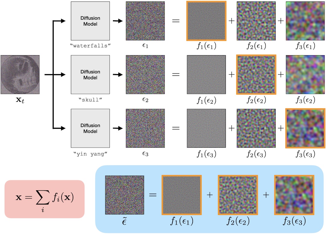
where \(\omega_t\) and \(\gamma_t\) are determined by the variance schedule and the scheduler. Then given a decomposition \( \mathbf{x} = \sum f_i(\mathbf{x}) \), this means the update rule can be decomposed into a sum of updates on components: \[ \begin{aligned} \mathbf{x}_{t-1} &= \texttt{update}(\mathbf{x}_t, \epsilon) \\ &= \texttt{update}\left( \sum f_i(\mathbf{x}_t), \sum f_i(\epsilon) \right) \\ &= \sum_i \texttt{update}(f_i(\mathbf{x}_t), f_i(\epsilon)) \end{aligned} \] where the last equality is by linearity of \( \texttt{update}(\cdot,\cdot) \). Our method can be understood as conditioning each of these components on a different text prompt. Written explicitly, for text prompts \( y_i \) our method is \[ \begin{aligned} \mathbf{x}_{t-1} = \sum_i \texttt{update}(f_i(\mathbf{x}_t), f_i(\epsilon(\mathbf{x}_t, y_i, t))). \end{aligned} \] Moreover, if the \( f_i \)'s are linear then we have \[ \begin{aligned} f_i(\mathbf{x}_{t-1}) &= f_i(\texttt{update}(\mathbf{x}_t, \epsilon)) \\ &= f_i(\omega_t\mathbf{x}_t + \gamma_t\epsilon_\theta) \\ &= \omega_t f_i(\mathbf{x}_t) + \gamma_t f_i(\epsilon_\theta) \\ &= \texttt{update}(f_i(\mathbf{x}_t), f_i(\epsilon_\theta)), \end{aligned} \] meaning that updating using the \(i\)th component of \(\mathbf{x}_t\) with the \(i\)th component of \(\epsilon_\theta\) will only affect the \(i\)th component of \(\mathbf{x}_{t-1}\).

1The update function also depends on \(t\), which we omit for brevity.

2Noise of the form \( \mathbf{z}\sim\mathcal{N}(0,\mathbf{I}) \) is also often added, which can be safely ignored. Please see the paper for details.

Inverse Problems

If we know what one of the components must be, perhaps from some reference image \( \mathbf{x}_\text{ref} \), then we can hold that component constant while generating the other components. In practice we do this by reprojecting the noisy image \( \mathbf{x}_t \) at every time step: \[ \mathbf{x}_t \gets f_1\left(\sqrt{\alpha_t}\mathbf{x}_\text{ref} + \sqrt{1 - \alpha_t}\epsilon\right) + \sum_{i=2}^N f_i(\mathbf{x}_t) \] This is effectively a way to solve (noiseless) inverse problems, with forward model \( \mathbf{y} = f_1(\mathbf{x}) \), and can be seen as a rudimentary version of prior work [4][5][6][7][8]. We apply this approach to generating hybrid images from real images, which we show above, and in a gallery of results.

Limitations and Random Results

One major limitation of our method is that the success rate is relatively low. While our method can produce decent images consistently, very high quality images are rarer. We attribute this fragility to the fact that our method produces images that are highly out-of-distribution for the diffusion model. In addition, there is no mechanism by which prompts associated with one component are discouraged from appearing in other components. Another failure case of our method is that the prompt for one component may dominate the generated image. Empirically, the success rate of our method can be improved by carefully choosing prompt pairs or by manually tuning decomposition parameters, but we leave improving the robustness of our method in general to future work. We show random results for selected prompt pairs below. Many more random results can be found in our paper.

Related Links

This project is related to a number of other works, including:

Recent work by a pseudonymous artist, Ugleh, uses a Stable Diffusion model finetuned for generating QR codes to produce images whose global structure subtly matches a given template image. These images can effectively act as hybrid images. A demo of this approach can be found here.

Prior work, Generative Powers of Ten by Xiaojuan Wang et al., first showed that an image could be denoised with different conditioning in different frequency subbands. They apply this to the task of generating extreme zooms of images, where a stack of images represents different zoom levels. Each zoom-level is then conditioned on a different prompt, with zoomed-out images serving as constraints on the low frequency components of zoomed-in images.

Work by Matthew Tancik, and our prior work, Visual Anagrams, show how to make illusions by denoising multiple views of an image simultaneously. These methods work by transforming the inputs to the diffusion model, while factorized diffusion modifies the outputs of the diffusion model, producing a different class of illusions.

Another approach to making illusions with diffusion models is to use score distillation sampling, which is done in Diffusion Illusions, by Ryan Burgert et al.

BibTeX

@article{geng2024factorized,
  title     = {Factorized Diffusion: Perceptual Illusions by Noise Decomposition},
  author    = {Geng, Daniel and Park, Inbum and Owens, Andrew},
  journal   = {arXiv:2404.11615},
  year      = {2024},
  month     = {April},
  abbr      = {Preprint},
  url       = {https://arxiv.org/abs/2404.11615},
}