Thin film interference seen in soap-bubbles is a time-variant process. Environmental forces like wind or gravity generate velocity fields in the bubble's membrane causing its thickness to vary spatially and temporally. As a result, in nature we often see a splendor of chromatic patterns evolving over a fluid surface.
Inspired by such beauty, we were interested in marrying fluid dynamics with thin film interference to render a simulation of this phenomenon. Here we implement a standalone fluid simulator on a spherical manifold and embed thin film interference functionality directly into the Project 3 Pathtracer codebase by creating a specialized BSDF. How these two elements connect is straightforward. At a high-level, our fluid simulator propagates a scalar quantity along a perscribed velocity vector field defined on the surface of the sphere. We interpret this scalar quantity as the thickness of the film at each point on the spherical bubble surface. As we render each frame, the pathtracer queries a thickness map at the point corresponding to the ray intersection location on the bubble. Using the thickness, the effect of interference for each RGB color channel can be calculated and conveyed to the ray. We demonstrate videos for two different refractive media comprising the bubble: an oily media and a soapy media.
1 Implementing Fluid Simulation on a Spherical Manifold (Technical Approach)
1.1 Fluid Dynamics Theory
The Navier-Stokes equations for incompressible fluids are a system of PDEs that describe the rate of change of a fluid's velocity vector field \( \mathbf{u} \).
where \( \nu = \frac{\mu}{\rho_0} \) is the kinematic fluid viscosity, \( \nabla^2 \mathbf{u} \) is the vector laplacian, and \( \mathbf{f} \) is a general force vector field encapsulating both internal and body forces. Generally, \( \mathbf{f} = -\nabla p + \mathbf{f_{ext}} \) where \( \nabla p \) is the density-normalized pressure gradient within the fluid and \( \mathbf{f_{ext}} \) is a density-normalized external force like gravity (e.g. \( \mathbf{f_{ext}} = \mathbf{g} \) ). Density-normalized simply means we've divided out both sides of equation by the fluid density \( \rho_0 \) so that the units are compatible. (Navier-Stokes Wiki). Equation 2 is simply a statement about the incompressibility of the fluid.
In practice, to visualize flow we need to consider the motion of a separate substance within the fluid like smoke or ink. The important feature of this substance is its density in every region of the fluid. This important scalar quantity is transported by the fluid velocity field and diffusion. Its evolution is characterized through Equation 3 below (note the symmetry between equations 1 and 3).
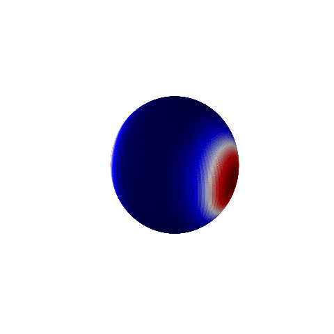
Note that the example of density transport is a tautology for the transport of any scalar field. For the purposes of our project, we consider the scalar field to be a thickness map for a thin film object. In other words, we consider the transport of "thickness" within the bubble membrane.
1.2 A First Pass at a Planar Simulator
Following [1] we implemented a basic planar fluid simulator with various boundary conditions.
Karman Vortex Sheets!
Kelvin-Helmholtz Instability!
Wrapped boundary conditions!
We implement this by maintaining both a scalar density field and a vector velocity field. Both are updated with a diffusion and advection solver. Diffsion is simulated by solving the poisson equation with gauss-seidel and advection is simulated by backtracing. In addition, at every step we ensure the incompressibility constraint by "projecting" the velocity field \( \mathbf{v} \). We do this by taking advantage of the Helmholtz decomposition, which states that any vector field (under sufficient conditions) can be written as the sum of a solenoidal (divergence-less) field and a conservative (curl-less) field:
where \(\mathbf{A}\) is the vector potential and \(\Phi\) is the scalar potential. Applying the divergence operator to both sides and using the fact that the divergence of a solenoidal field is 0 we have
This gives us a poisson equation that we can again solve using gauss-seidel, giving us the scalar potential. Subtracting off the gradient of this potential gives us the desired solenoidal projection. Different boundary conditions can be implemented by modifying the gauss-seidel solvers and the backtracing step.
1.3 Adapting Planar Simulator to a Spherical Manifold
To simulate fluids on a sphere we took two approaches. The first approach involved simply warping the results of a planar simulator on to a sphere. In the second approach we build a native spherical fluid simulator.
The first approach is easy, but doesn't produce good results near the poles (or wherever the singularity of the warping transform is). We use a simple longitude-latitude map and get the following result.
Projective texture map to sphere
Notice here we specifically use a fluid flow that vanishes near the poles
The second approach involves natively simulating the fluid on a sphere. This requires numerically solving the Navier-Stokes PDEs in spherical coordinates. To do this we used the Chebfun library in Matlab. The library is fairly stable (depending on the discretization) so we avoid problems with singularities at the poles. Our implementation yielded the following results:
Native Spherical Fluid Simulator.
Finally, in order to feed these simulations to the ray tracer we embed the density field for each frame into a .DAE file template and save to disk. This .DAE file is later read by the pathtracer when constructing the thin film BSDF objects (See DAE File Guide for details).
2 Implementing Thin Film Interference (Technical Approach)
2.1 Thin Film Interference Theory
Thin film interference is fundamentally a result of the wave-like nature of light. Light incident on a transmissive thin film surface undergoes both reflection and refraction. The refracted portion has an additional opportunity to reflect at the second interface of the thin film. The phase difference between these two reflections induces either constructive or destructive interference. The fractional intensities of the total transmitted and reflected light for given wavelength are defined as:
where \(\alpha\) and \(\beta\) are related to the Fresnel coefficients as described in [4] and \(\varphi\) is the phase difference between the two reflections (See Thin Film Derivation for a complete derivation).
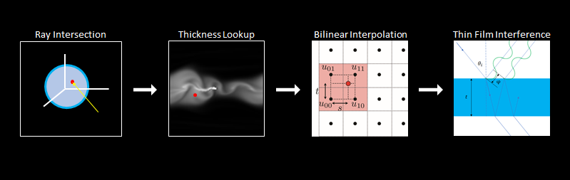
The phase difference \(\varphi\) is the crux of this visual phenomena. Importantly, it is dependent on the wavelength \(\lambda\) of the incident light, as well as the thickness \(\delta\) of the thin film. This quantity \(\delta\) is precisely what we query from the 2D fluid simulator at each ray intersection with the bubble. To reemphasize, the thickness of the film is a function of position over the bubble surface for a given instant in time. As the thickness map is a discrete grid, use bilinear interpolation to distill the appropriate thickness for ray intersections that do not map precisely onto grid points. Finally, we restrict our implementation of thin film interactions to systems containing only two material interfaces. Hence, there are a maximum of three refractive indices \(n_1, n_2,\) and \(n_3\) involved in any calculation.
2.2 Thin Film BSDFS
Our initial implementation of thin film phenomena closely followed the routines described in [4] for discerning the fractional intensities of reflected and transmitted light on a thin film surface. The relevant parameters are the incident angle of the ray, the wavelength corresponding to each color channel, the refractive index of the thin film media at each wavelength, and the film thickness at the intersection point. Having implemented a refractive BSDF already in Assignment 3-2, we structured our new BSDF's ray sampling function after the Glass BSDF which takes a probablistic approach to reflection and transmission. Importantly, the constructor for the thin film BSDF assigns a pointer to the thickness map generated by the fluid simulator and stores the refractive indices of the internal and surrounding media.
2.3 Interference Calculation Pipeline
Consider a ray intersecting with a bubble object - an sphere in the scene which has been paired with our thin film BSDF. The intersection location can be mapped directly to a location on the thickness map generated by the fluid simulator. The thickness value used for calculating thin film interference effects on this ray is taken to be a bilinear interpolation of the thickness values corresponding to the four nearest discrete grid points. Using this thickness value we compute the transmission and reflection coefficients for each RGB channel (as interference is wavelength dependent) and convey this information to the ray.
Diagram showing procedure for calculating interference effects.
2.4 Pseudo-Physical Interference
After ending up with unrealistic renders in our initial thin film interference implementation, we resorted to a pseudo-physical interference scheme that departs slightly from the theory presented in section 2.1.
Instead, we use the Schlick Approximation to the Fresnel Factor scaled by a wavelength-dependent weighting term. While physically inaccurate, this method produced more realistic results.
\begin{equation} \tag{9} \label{eq: pseudo-physical}
R_\lambda = w_\lambda \cdot R_s
\end{equation}
\begin{equation} \tag{10} \label{eq: pseudo-physical-specifics}
w_\lambda = \frac{ 1 + \cos(\varphi)}{2} \hspace{2cm} \text{ and } \hspace{2cm} \varphi = \frac{2 \pi}{\lambda}(\frac{2 n_1 \delta}{\cos(\theta_i)} + \Delta)
\end{equation}
3 Results
3.1 Thin Film Interference Videos
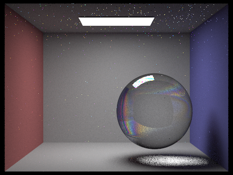
Here we present videos of our results for two types of thin film media: oil and soap. In an effort to limit lengthy render times, we ran our pathtracer with the following settings: 256 ray samples per pixel, adaptive sampling thresholded at 0.05, and a ray depth of 5. Under these settings, it took our pathtracer about two hours to render all 100 frames comprising each video.
Oily Thin Film Example 1
Oily Thin Film Example 2
Soapy Thin Film Example 1
Soapy Thin Film Example 2
3.2 Denoising Renders
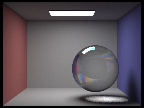
An issue we enountered in our frame renders was impulse noise. This noise was inconsistent from frame to frame and produced distracting artifacts in the videos. In response to this, we decided to apply a median kernel for denoising each frame. This 3x3 kernel assigns the center pixel to the median value of the surrounding pixels. Since it is in the nature of impulse noise to occur primarily over the span of a single pixel, this filtering technique was incredibly effective as shown in the comparison renders below. Consequently, we applied this filter to each frame of our thin film videos.
Impulse Noise in Renders
Denoising with Median Filter Kernel
4 Contributions From Each Team Member
Daniel: I worked on implementing both the planar and spherical fluid simulator from scratch. In addition I helped generate some DAE files from the simulator results
Nico: I worked on building and integrating the thin film BSDF in the project 3 codebase. I also modified the COLLADA parsers to read fluid simulator data and designed a .DAE file template to interface our fluid simulator with our pathtracer. Finally, I worked on denoising the final renders.
Efficient Fluid Simulation on the Surface of a Sphere, David J. Hill, Ronald D. Henderson. DreamWorks Animation.
Real-Time Fluid Simulation on the Surface of a Sphere, Bowen Yang, William Corse, Jiecong Lu, Joshuah Wolper, Chenfanfu Jiang. University Pennsylvania.
Fluid Dynamics. Steve Rotenberg. UC San Diego CE 169 Computer Animation, 2016.